Civilpy - 文章

Bokeh视觉属性（核心）

发布时间：2021-12-03 公开文章

1.使用色盘

>>> from bokeh.palettes import Spectral6
>>> Spectral6
['#3288bd', '#99d594', '#e6f598', '#fee08b', '#fc8d59', '#d53e4f']

bokeh.palettes - Bokeh 1.0.2 documentationbokeh.pydata.org/en/latest/docs/reference/palettes.html

2.使用映射器

bokeh.transform.factor_cmap
bokeh.transform.linear_cmap
bokeh.transform.log_cmap

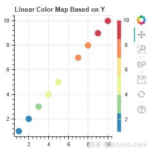
from bokeh.plotting import figure, show, output_file
from bokeh.models import ColumnDataSource, ColorBar
from bokeh.palettes import Spectral6
from bokeh.transform import linear_cmap

output_file("styling_linear_mappers.html", title="styling_linear_mappers.py example")

x = [1,2,3,4,5,7,8,9,10]
y = [1,2,3,4,5,7,8,9,10]

#Use the field name of the column source
# 根据y轴数据进行映射
mapper = linear_cmap(field_name='y', palette=Spectral6 ,low=min(y) ,high=max(y))

source = ColumnDataSource(dict(x=x,y=y))

p = figure(plot_width=300, plot_height=300, title="Linear Color Map Based on Y")

p.circle(x='x', y='y', line_color=mapper,color=mapper, fill_alpha=1, size=12, source=source)

# 增加色轴
color_bar = ColorBar(color_mapper=mapper['transform'], width=8,  location=(0,0))

# 设置色轴的位置
p.add_layout(color_bar, 'right')

show(p)

3.视觉特性

3.1 Line Properties（线条特性）

line_color、line_width、line_alpha、line_dash、line_dash_offset。

3.2Fill Properties（填充特性）

fill_color、fill_alpha

3.3Text Properties（文本特性）

text_font、text_font_size、text_font_style、text_color、text_alpha、text_align、text_baseline

4.可视特性

4.1 线条或坐标轴可视

from bokeh.io import output_file, show
from bokeh.plotting import figure

# We set-up a standard figure with two lines
p = figure(plot_width=500, plot_height=200, tools='')
visible_line = p.line([1, 2, 3], [1, 2, 1], line_color="blue")
invisible_line = p.line([1, 2, 3], [2, 1, 2], line_color="pink")

# We hide the xaxis, the xgrid lines, and the pink line
invisible_line.visible = False
p.xaxis.visible = False
p.xgrid.visible = False

output_file("styling_visible_property.html")

show(p)

4.2Specifying Colors（指定颜色）

147 种 CSS颜色，例如 'green', 'indigo'
16位RGB色值，例如 '#FF0000', '#44444444'
3数元组 (r,g,b) ，整型数据0 到 255
4数元组(r,g,b,a) ，增加最后一位透明度介于0到1

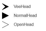
4.3Styling Arrow Annotations（注释箭头）

4.4Screen Units and Data-space Units（屏幕单位和绘图空间单位）

屏幕单元使用原始像素数来指定高度或宽度，而数据空间单元相对于数据和图的轴。例如，在一个400像素×400像素、x轴和y轴从0到10的图形中，宽度和高度为图形五分之一的字形将是80个屏幕单元或2个数据空间单元。

5.画布属性

画布对象本身具有许多可样式化的视觉特征:情节的维度、背景、边框、轮廓等等。

http://bokeh.pydata.org/en/latest/docs/reference/plotting.html#bokeh-plottingbokeh.pydata.org/en/latest/docs/reference/plotting.html#bokeh-plotting

bokeh.plotting - Bokeh 1.0.2 documentation

bokeh.plotting - Bokeh 1.0.2 documentationbokeh.pydata.org/en/latest/docs/reference/plotting.html#bokeh-plotting

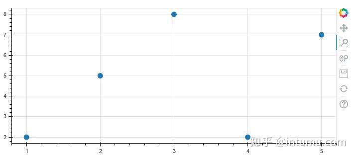
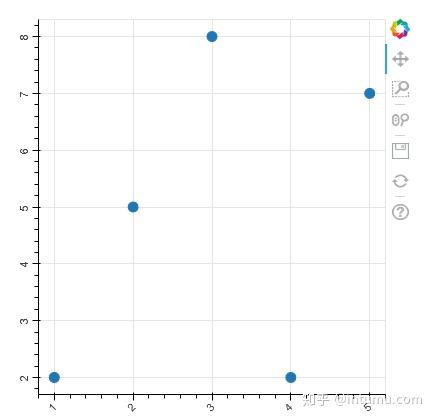
5.1Dimensions（维度）

from bokeh.plotting import figure, output_file, show

output_file("dimensions.html")

# create a new plot with specific dimensions
p = figure(plot_width=700)
p.plot_height = 300

p.circle([1, 2, 3, 4, 5], [2, 5, 8, 2, 7], size=10)

show(p)

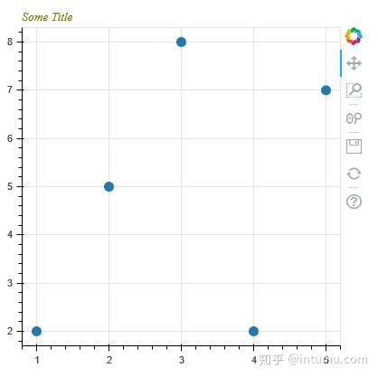
5.2Title（标题）

from bokeh.plotting import figure, output_file, show

output_file("title.html")

p = figure(plot_width=400, plot_height=400, title="Some Title")
p.title.text_color = "olive"
p.title.text_font = "times"
p.title.text_font_style = "italic"

p.circle([1, 2, 3, 4, 5], [2, 5, 8, 2, 7], size=10)

show(p)

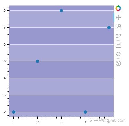
5.3Background（背景）

from bokeh.plotting import figure, output_file, show

output_file("background.html")

p = figure(plot_width=400, plot_height=400)
p.background_fill_color = "beige"
p.background_fill_alpha = 0.5

p.circle([1, 2, 3, 4, 5], [2, 5, 8, 2, 7], size=10)

show(p)

5.4Border（边框）

from bokeh.plotting import figure, output_file, show

output_file("border.html")

p = figure(plot_width=400, plot_height=400)
p.border_fill_color = "whitesmoke"
p.min_border_left = 80

p.circle([1,2,3,4,5], [2,5,8,2,7], size=10)

show(p)

5.5Outline(轮廓)

from bokeh.plotting import figure, output_file, show

output_file("outline.html")

p = figure(plot_width=400, plot_height=400)
p.outline_line_width = 7
p.outline_line_alpha = 0.3
p.outline_line_color = "navy"

p.circle([1,2,3,4,5], [2,5,8,2,7], size=10)

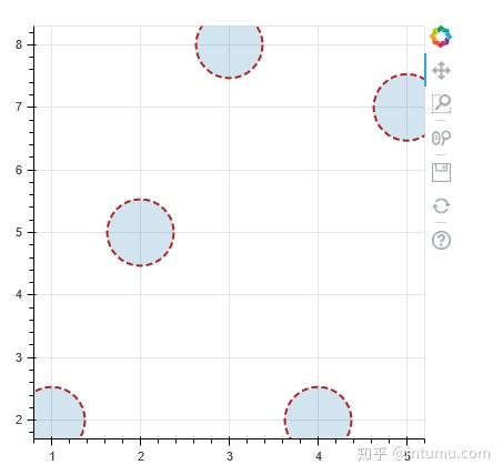
show(p)

6.图元属性（重点）

from bokeh.plotting import figure, output_file, show

output_file("axes.html")

p = figure(plot_width=400, plot_height=400)
r = p.circle([1,2,3,4,5], [2,5,8,2,7])

glyph = r.glyph
glyph.size = 60
glyph.fill_alpha = 0.2
glyph.line_color = "firebrick"
glyph.line_dash = [6, 3]
glyph.line_width = 2

show(p)

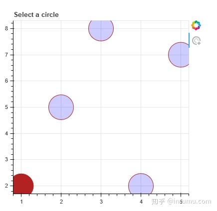
6.1选择或取消选择图元

from bokeh.io import output_file, show
from bokeh.plotting import figure
from bokeh.models import Circle

output_file("styling_selections.html")

plot = figure(plot_width=400, plot_height=400, tools="tap", title="Select a circle")
renderer = plot.circle([1, 2, 3, 4, 5], [2, 5, 8, 2, 7], size=50)

selected_circle = Circle(fill_alpha=1, fill_color="firebrick", line_color=None)
nonselected_circle = Circle(fill_alpha=0.2, fill_color="blue", line_color="firebrick")

renderer.selection_glyph = selected_circle
renderer.nonselection_glyph = nonselected_circle

show(plot)

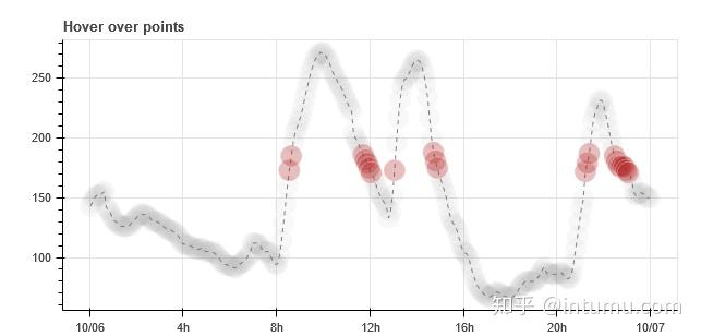
6.2鼠标悬停检查

from bokeh.plotting import figure, output_file, show
from bokeh.models import HoverTool
from bokeh.sampledata.glucose import data

output_file("styling_hover.html")

subset = data.loc['2010-10-06']

x, y = subset.index.to_series(), subset['glucose']

# Basic plot setup
plot = figure(plot_width=600, plot_height=300, x_axis_type="datetime", tools="",
              toolbar_location=None, title='Hover over points')

plot.line(x, y, line_dash="4 4", line_width=1, color='gray')

cr = plot.circle(x, y, size=20,
                fill_color="grey", hover_fill_color="firebrick",
                fill_alpha=0.05, hover_alpha=0.3,
                line_color=None, hover_line_color="white")

plot.add_tools(HoverTool(tooltips=None, renderers=[cr], mode='hline'))

show(plot)

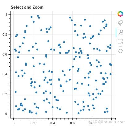
6.3Tool Overlays（工具栏）

import numpy as np

from bokeh.models import BoxSelectTool, BoxZoomTool, LassoSelectTool
from bokeh.plotting import figure, output_file, show

output_file("styling_tool_overlays.html")

x = np.random.random(size=200)
y = np.random.random(size=200)

# Basic plot setup
plot = figure(plot_width=400, plot_height=400, title='Select and Zoom',
              tools="box_select,box_zoom,lasso_select,reset")

plot.circle(x, y, size=5)

select_overlay = plot.select_one(BoxSelectTool).overlay

select_overlay.fill_color = "firebrick"
select_overlay.line_color = None

zoom_overlay = plot.select_one(BoxZoomTool).overlay

zoom_overlay.line_color = "olive"
zoom_overlay.line_width = 8
zoom_overlay.line_dash = "solid"
zoom_overlay.fill_color = None

plot.select_one(LassoSelectTool).overlay.line_dash = [10, 10]

show(plot)

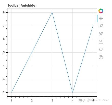
6.4 工具栏自动隐藏

from bokeh.plotting import figure, output_file, show

output_file("styling_toolbar_autohide.html")

# Basic plot setup
plot = figure(width=400, height=400, title='Toolbar Autohide')
plot.line([1,2,3,4,5], [2,5,8,2,7])

# Set autohide to true to only show the toolbar when mouse is over plot
plot.toolbar.autohide = True

show(plot)

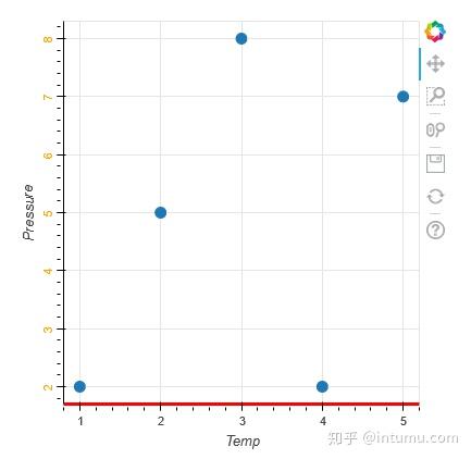
6.4坐标轴

from bokeh.plotting import figure, output_file, show

output_file("axes.html")

p = figure(plot_width=400, plot_height=400)
p.circle([1,2,3,4,5], [2,5,8,2,7], size=10)

# change just some things about the x-axes
p.xaxis.axis_label = "Temp"
p.xaxis.axis_line_width = 3
p.xaxis.axis_line_color = "red"

# change just some things about the y-axes
p.yaxis.axis_label = "Pressure"
p.yaxis.major_label_text_color = "orange"
p.yaxis.major_label_orientation = "vertical"

# change things on all axes
p.axis.minor_tick_in = -3
p.axis.minor_tick_out = 6

show(p)

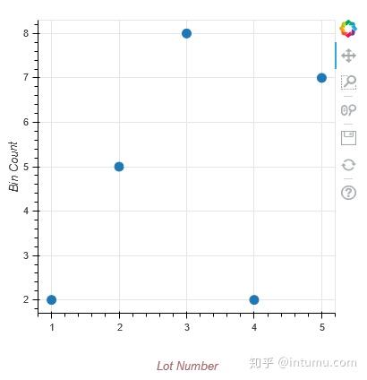
6.5 标签

from bokeh.plotting import figure, output_file, show

output_file("bounds.html")

p = figure(plot_width=400, plot_height=400)
p.circle([1,2,3,4,5], [2,5,8,2,7], size=10)

p.xaxis.axis_label = "Lot Number"
p.xaxis.axis_label_text_color = "#aa6666"
p.xaxis.axis_label_standoff = 30

p.yaxis.axis_label = "Bin Count"
p.yaxis.axis_label_text_font_style = "italic"

show(p)

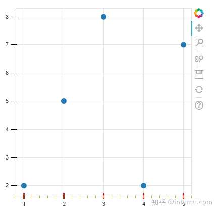
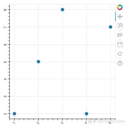
6.6Bounds（坐标轴界限）

from bokeh.plotting import figure, output_file, show

output_file("bounds.html")

p = figure(plot_width=400, plot_height=400)
p.circle([1,2,3,4,5], [2,5,8,2,7], size=10)

p.xaxis.bounds = (2, 4)

show(p)

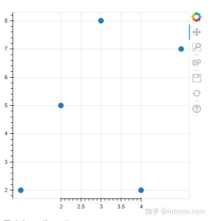
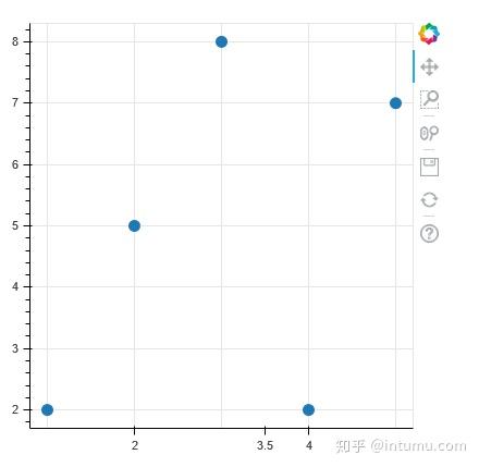
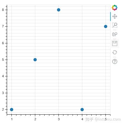
6.7Tick Locations（坐标轴刻度标记）

from bokeh.plotting import figure, output_file, show

output_file("fixed_ticks.html")

p = figure(plot_width=400, plot_height=400)
p.circle([1,2,3,4,5], [2,5,8,2,7], size=10)

p.xaxis.ticker = [2, 3.5, 4]

show(p)

6.7刻度线

from bokeh.plotting import figure, output_file, show

output_file("axes.html")

p = figure(plot_width=400, plot_height=400)
p.circle([1,2,3,4,5], [2,5,8,2,7], size=10)

p.xaxis.major_tick_line_color = "firebrick"
p.xaxis.major_tick_line_width = 3
p.xaxis.minor_tick_line_color = "orange"

p.yaxis.minor_tick_line_color = None

p.axis.major_tick_out = 10
p.axis.minor_tick_in = -3
p.axis.minor_tick_out = 8

show(p)

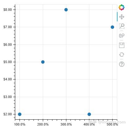
6.8刻度标记格式

from bokeh.plotting import figure, output_file, show
from bokeh.models import NumeralTickFormatter

output_file("gridlines.html")

p = figure(plot_width=400, plot_height=400)
p.circle([1,2,3,4,5], [2,5,8,2,7], size=10)

p.xaxis[0].formatter = NumeralTickFormatter(format="0.0%")
p.yaxis[0].formatter = NumeralTickFormatter(format="$0.00")

show(p)

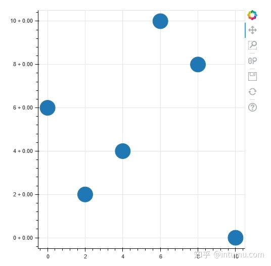
from bokeh.models import FuncTickFormatter
from bokeh.plotting import figure, show, output_file

output_file("formatter.html")

p = figure(plot_width=500, plot_height=500)
p.circle([0, 2, 4, 6, 8, 10], [6, 2, 4, 10, 8, 0], size=30)

p.yaxis.formatter = FuncTickFormatter(code="""
    return Math.floor(tick) + " + " + (tick % 1).toFixed(2)
""")

show(p)

6.9Tick Label Orientation(标记角度)

from math import pi
from bokeh.plotting import figure, output_file, show

output_file("gridlines.html")

p = figure(plot_width=400, plot_height=400)
p.circle([1,2,3,4,5], [2,5,8,2,7], size=10)

p.xaxis.major_label_orientation = pi/4
p.yaxis.major_label_orientation = "vertical"

show(p)

6.10网格

from math import pi
from bokeh.plotting import figure, output_file, show

output_file("gridlines.html")

p = figure(plot_width=400, plot_height=400)
p.circle([1,2,3,4,5], [2,5,8,2,7], size=10)

p.xaxis.major_label_orientation = pi/4
p.yaxis.major_label_orientation = "vertical"

show(p)

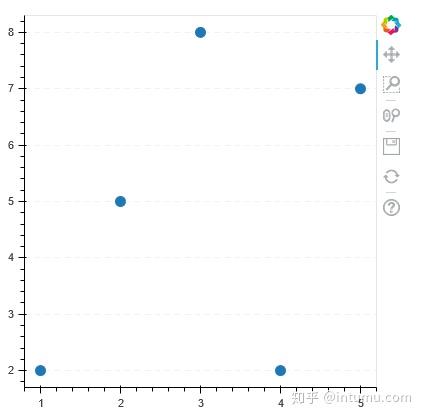
6.11Grids（网格）

from bokeh.plotting import figure, output_file, show

output_file("gridlines.html")

p = figure(plot_width=400, plot_height=400)
p.circle([1,2,3,4,5], [2,5,8,2,7], size=10)

# change just some things about the x-grid
p.xgrid.grid_line_color = None

# change just some things about the y-grid
p.ygrid.grid_line_alpha = 0.5
p.ygrid.grid_line_dash = [6, 4]

show(p)

网格小行

from bokeh.plotting import figure, output_file, show

output_file("minorgridlines.html")

p = figure(plot_width=400, plot_height=400)
p.circle([1,2,3,4,5], [2,5,8,2,7], size=10)

# change just some things about the y-grid
p.ygrid.minor_grid_line_color = 'navy'
p.ygrid.minor_grid_line_alpha = 0.1

show(p)

from bokeh.plotting import figure, output_file, show

output_file("gridbands.html")

p = figure(plot_width=400, plot_height=400)
p.circle([1,2,3,4,5], [2,5,8,2,7], size=10)

# change just some things about the x-grid
p.xgrid.grid_line_color = None

# change just some things about the y-grid
p.ygrid.band_fill_alpha = 0.1
p.ygrid.band_fill_color = "navy"

show(p)

from bokeh.plotting import figure, output_file, show

output_file("bounds.html")

p = figure(plot_width=400, plot_height=400)
p.circle([1,2,3,4,5], [2,5,8,2,7], size=10)

p.grid.bounds = (2, 4)

show(p)

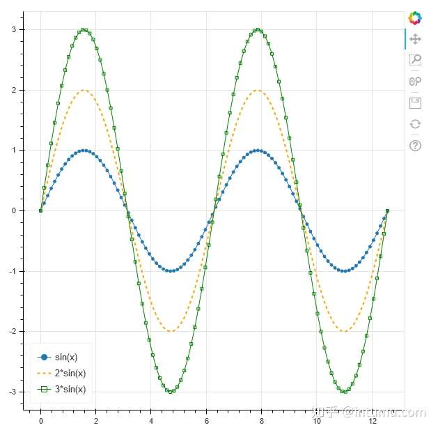
7Legends（图例）

7.1Location（位置）

import numpy as np
from bokeh.plotting import figure, show, output_file

x = np.linspace(0, 4*np.pi, 100)
y = np.sin(x)

output_file("legend_labels.html")

p = figure()

p.circle(x, y, legend="sin(x)")
p.line(x, y, legend="sin(x)")

p.line(x, 2*y, legend="2*sin(x)",
       line_dash=[4, 4], line_color="orange", line_width=2)

p.square(x, 3*y, legend="3*sin(x)", fill_color=None, line_color="green")
p.line(x, 3*y, legend="3*sin(x)", line_color="green")

p.legend.location = "bottom_left"

show(p)

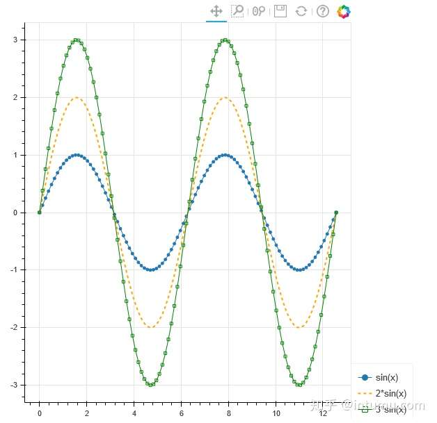
7.2Outside the Plot Area（显示至画布外）

import numpy as np
from bokeh.models import Legend
from bokeh.plotting import figure, show, output_file

x = np.linspace(0, 4*np.pi, 100)
y = np.sin(x)

output_file("legend_labels.html")

p = figure(toolbar_location="above")

r0 = p.circle(x, y)
r1 = p.line(x, y)

r2 = p.line(x, 2*y, line_dash=[4, 4], line_color="orange", line_width=2)

r3 = p.square(x, 3*y, fill_color=None, line_color="green")
r4 = p.line(x, 3*y, line_color="green")

legend = Legend(items=[
    ("sin(x)"   , [r0, r1]),
    ("2*sin(x)" , [r2]),
    ("3*sin(x)" , [r3, r4]),
], location=(0, -30))

p.add_layout(legend, 'right')

show(p)

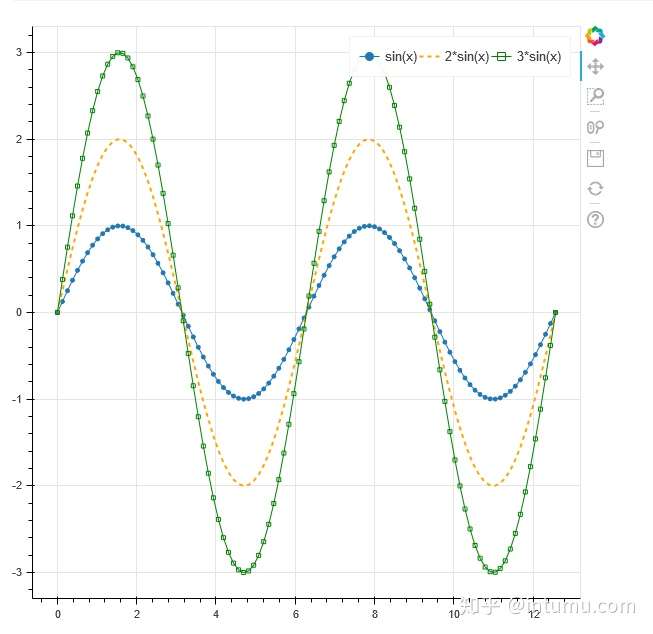
7.3Orientation（方向）

import numpy as np
from bokeh.plotting import figure, show, output_file

x = np.linspace(0, 4*np.pi, 100)
y = np.sin(x)

output_file("legend_labels.html")

p = figure()

p.circle(x, y, legend="sin(x)")
p.line(x, y, legend="sin(x)")

p.line(x, 2*y, legend="2*sin(x)",
       line_dash=[4, 4], line_color="orange", line_width=2)

p.square(x, 3*y, legend="3*sin(x)", fill_color=None, line_color="green")
p.line(x, 3*y, legend="3*sin(x)", line_color="green")

p.legend.orientation = "horizontal"

show(p)

7.4Label Text（图例文本）

import numpy as np
from bokeh.plotting import output_file, figure, show

x = np.linspace(0, 4*np.pi, 100)
y = np.sin(x)

output_file("legend_labels.html")

p = figure()

p.circle(x, y, legend="sin(x)")
p.line(x, y, legend="sin(x)")

p.line(x, 2*y, legend="2*sin(x)",
       line_dash=[4, 4], line_color="orange", line_width=2)

p.square(x, 3*y, legend="3*sin(x)", fill_color=None, line_color="green")
p.line(x, 3*y, legend="3*sin(x)", line_color="green")

p.legend.label_text_font = "times"
p.legend.label_text_font_style = "italic"
p.legend.label_text_color = "navy"

show(p)

7.5Border（边框）

import numpy as np
from bokeh.plotting import output_file, figure, show

x = np.linspace(0, 4*np.pi, 100)
y = np.sin(x)

output_file("legend_border.html")

p = figure()

p.circle(x, y, legend="sin(x)")
p.line(x, y, legend="sin(x)")

p.line(x, 2*y, legend="2*sin(x)",
       line_dash=[4, 4], line_color="orange", line_width=2)

p.square(x, 3*y, legend="3*sin(x)", fill_color=None, line_color="green")
p.line(x, 3*y, legend="3*sin(x)", line_color="green")

p.legend.border_line_width = 3
p.legend.border_line_color = "navy"
p.legend.border_line_alpha = 0.5

show(p)

7.6背景

import numpy as np
from bokeh.plotting import output_file, figure, show

x = np.linspace(0, 4*np.pi, 100)
y = np.sin(x)

output_file("legend_background.html")

p = figure()

p.circle(x, y, legend="sin(x)")
p.line(x, y, legend="sin(x)")

p.line(x, 2*y, legend="2*sin(x)",
       line_dash=[4, 4], line_color="orange", line_width=2)

p.square(x, 3*y, legend="3*sin(x)", fill_color=None, line_color="green")
p.line(x, 3*y, legend="3*sin(x)", line_color="green")

#  3*sin(x) curve should be under this legend at initial viewing, so
# we can see that the legend is transparent
p.legend.location = "bottom_right"
p.legend.background_fill_color = "navy"
p.legend.background_fill_alpha = 0.5

show(p)