某国外电商销售数据分析之客户留存(含源码及数据源)
发布时间:2021-12-04
付费文章:2.0元
Talk is cheap
import pandas as pd
import numpy as np
from datetime import datetime
import matplotlib as mpl
import matplotlib.pyplot as plt
pd.set_option('display.max_columns', 20)
pd.set_option('display.max_rows', 10)


plt.rcParams['font.sans-serif'] = ['SimHei']  # 用来正常显示中文标签
plt.rcParams['axes.unicode_minus'] = False #当坐标轴有负号的时候可以显示负号
%matplotlib inline
Cohort Analysis 留存分析
http://www.woshipm.com/data-analysis/712880.html
准备数据
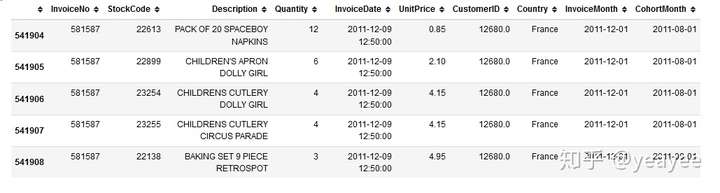
online=pd.read_csv("../data/数据源见页底.csv",parse_dates=['InvoiceDate'])  # 直接将'InvoiceDate'列转为时间格式
online.head()
online.info()
<class 'pandas.core.frame.DataFrame'>
RangeIndex: 541909 entries, 0 to 541908
Data columns (total 8 columns):
 #   Column       Non-Null Count   Dtype
---  ------       --------------   -----
 0   InvoiceNo    541909 non-null  object
 1   StockCode    541909 non-null  object
 2   Description  540455 non-null  object
 3   Quantity     541909 non-null  int64
 4   InvoiceDate  541909 non-null  datetime64[ns]
 5   UnitPrice    541909 non-null  float64
 6   CustomerID   406829 non-null  float64
 7   Country      541909 non-null  object
dtypes: datetime64[ns](1), float64(2), int64(1), object(4)
memory usage: 33.1+ MB
按首次购买月构建cohort
def get_month(x):
    return datetime(x.year, x.month,1)
online['InvoiceDate'].apply(get_month)
0        2010-12-01
1        2010-12-01
2        2010-12-01
3        2010-12-01
4        2010-12-01
            ...
541904   2011-12-01
541905   2011-12-01
541906   2011-12-01
541907   2011-12-01
541908   2011-12-01
Name: InvoiceDate, Length: 541909, dtype: datetime64[ns]
online['InvoiceMonth'] = online['InvoiceDate'].apply(get_month) # 将'InvoiceDate'返回为当月1号月初
online.head()
grouping = online.groupby('CustomerID')['InvoiceMonth']
grouping = online.groupby('CustomerID')['InvoiceMonth']
online['CohortMonth'] = grouping.transform('min') # 以用户ID转换该用户初次购买时间
online.tail()
获取cohort的索引
def get_date_int(df, column):
    year = df[column].dt.year
    month = df[column].dt.month
    day = df[column].dt.day
    return year, month, day
cohort_year,cohort_month,_=get_date_int(online, 'CohortMonth')
invoice_year, invoice_month,_ = get_date_int(online, 'InvoiceDate')
years_diff = invoice_year - cohort_year
months_diff = invoice_month - cohort_month
online['CohortPeriod'] = years_diff * 12 + months_diff + 1  # 第一个用户有活跃5个月
online.tail()
统计每个cohort的每月活跃用户数
online['Cohort']=online['CohortMonth'].astype(str)
online['Cohort']=online['Cohort'].apply(lambda x:x[:-3])
online.head()
grouping = online.groupby(['Cohort', 'CohortPeriod'])
cohort_data = grouping['CustomerID'].apply(pd.Series.nunique) #活跃用户
cohort_data = cohort_data.reset_index()
cohort_data.head()
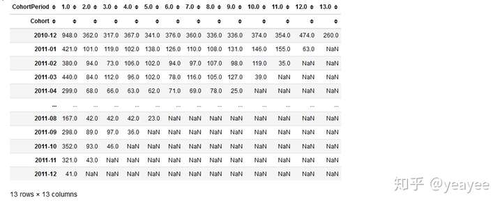
cohort_counts = cohort_data.pivot(index='Cohort',
columns='CohortPeriod',
values='CustomerID')
cohort_counts
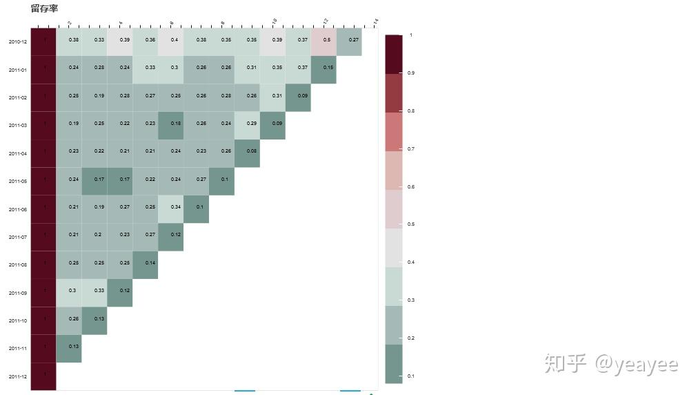
留存率(retention rate)
cohort_sizes = cohort_counts.iloc[:,0] # 用第一列数据对比计算留存率,归一化
retention = cohort_counts.divide(cohort_sizes, axis=0)
retention.head()
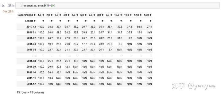
retention.round(3)*100
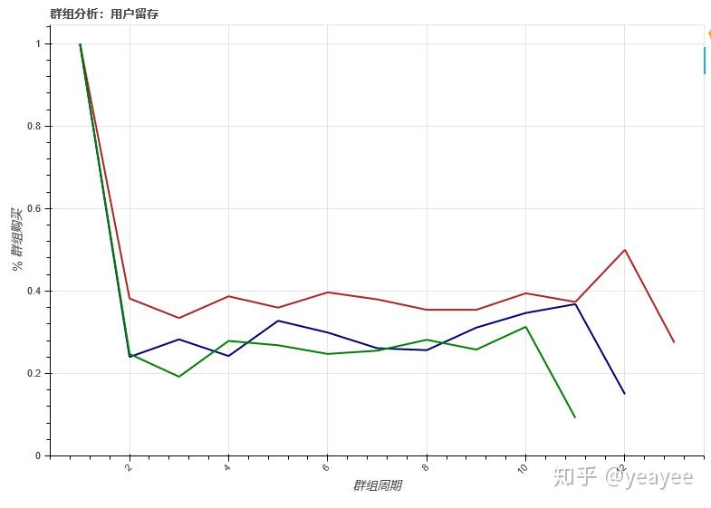
可视化cohort
retention.iloc[[0,1,2],:].T
from bokeh.plotting import figure, show, output_notebook
from bokeh.layouts import gridplot
from bokeh.models import ColumnDataSource,SingleIntervalTicker,FactorRange
from math import pi
output_notebook()
<div class="bk-root">
    <a href="https://bokeh.pydata.org" target="_blank" class="bk-logo bk-logo-small bk-logo-notebook"></a>
    <span id="1001">Loading BokehJS ...</span>
</div>
source = retention.iloc[[0,1,2],:].T
p = figure(plot_width=800, plot_height=550,title="群组分析:用户留存")
p.line(x='CohortPeriod',y='2010-12',color="firebrick",line_width=2,source=source)
p.line(x='CohortPeriod',y='2011-01',color="navy",line_width=2,source=source)
p.line(x='CohortPeriod',y='2011-02',color="green",line_width=2,source=source)
p.xaxis.axis_label = '群组周期'
p.yaxis.axis_label = '% 群组购买'
p.xaxis.major_label_orientation=pi/4
p.y_range.start=0
show(p)
打赏2.0元
手机端:用系统浏览器访问本链接,打开支付宝完成打赏
订单号示例
1.微信中:截图保存支付宝绿码,支付宝扫码打赏,手动获取;
2.电脑端:使用手机支付宝直接扫绿码,完成打赏,自动获取;