import tushare as ts
pro = ts.pro_api('******************')  # 到tushare官网注册账号获取token
ts_code = '300750'  # 600600  .SH .SZ 工业富联601138 贵州茅台600519 宁德时代300750
ts_code = ts_code+'.SZ'
ts_code
'300750.SZ'
df = pro.daily(ts_code=ts_code, start_date='20210101', end_date='20210531')
df.head()

# 将日期设为索引
df.index = pd.to_datetime(df['trade_date'], format='%Y%m%d')

# 导入及处理数据
import pandas as pd
import numpy as np
# 绘图
import matplotlib.pyplot as plt
# 设置图像标签显示中文
plt.rcParams['font.sans-serif'] = ['SimHei']
plt.rcParams['axes.unicode_minus'] = False
import matplotlib as mpl
# 解决一些编辑器(VSCode)或IDE(PyCharm)等存在的图片显示问题，
# 应用Tkinter绘图，以便对图形进行放缩操作
mpl.use('TkAgg')
%matplotlib inline
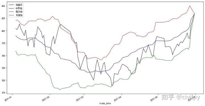
# SMA:简单移动平均(Simple Moving Average)
time_period = 20  # SMA的计算周期，默认为20
stdev_factor = 2  # 上下频带的标准偏差比例因子
history = []  # 每个计算周期所需的价格数据
sma_values = []  # 初始化SMA值
upper_band = []  # 初始化阻力线价格
lower_band = []  # 初始化支撑线价格

# 构造列表形式的绘图数据
for close_price in df['close']:
    # 
    history.append(close_price)

    # 计算移动平均时先确保时间周期不大于20
    if len(history) > time_period:
        del (history[0])

    # 将计算的SMA值存入列表
    sma = np.mean(history)
    sma_values.append(sma)  
    # 计算标准差
    stdev = np.sqrt(np.sum((history - sma) ** 2) / len(history))  
    upper_band.append(sma + stdev_factor * stdev)
    lower_band.append(sma - stdev_factor * stdev)
# 将计算的数据合并到DataFrame
df = df.assign(收盘价=pd.Series(df['close'], index=df.index))
df = df.assign(中界线=pd.Series(sma_values, index=df.index))
df = df.assign(阻力线=pd.Series(upper_band, index=df.index))
df = df.assign(支撑线=pd.Series(lower_band, index=df.index))
# 绘图
ax = plt.figure(figsize=(15, 8))
# 设定y轴标签
ax.ylabel = '%s price in ￥' % (ts_code)

df['收盘价'].plot(color='k', lw=1., legend=True)
df['中界线'].plot(color='b', lw=1., legend=True)
df['阻力线'].plot(color='r', lw=1., legend=True)
df['支撑线'].plot(color='g', lw=1., legend=True)
plt.show()

df.head()

from bokeh.plotting import figure, show

# Define Bollinger Bands.
upperband = df['阻力线']
lowerband = df['支撑线']
x_data = df.index

# Bollinger shading glyph:
band_x = np.append(x_data, x_data[::-1])
band_y = np.append(lowerband, upperband[::-1])

# output_file('bollinger.html', title='Bollinger bands (file)')

p = figure(x_axis_type='datetime', title="Bollinger Bands")
p.grid.grid_line_alpha = 0.4
p.x_range.range_padding = 0
p.plot_height = 600
p.plot_width = 800

p.patch(band_x, band_y, color='#7570B3', fill_alpha=0.2)  # 填充补丁，填充颜色透明度等

from bokeh.io import output_notebook, show
output_notebook()
show(p)
<div class="bk-root">
    <a href="https://bokeh.org" target="_blank" class="bk-logo bk-logo-small bk-logo-notebook"></a>
    <span id="1175">Loading BokehJS ...</span>
</div>

# 年化收益率
annual_profit=(1+(df.head(1)['close'].values[0]/df.tail(1)['close'].values[0]-1))**(250/df.shape[0])-1
annual_profit
0.2026992772623244
# 最大回撤
highest_close=df['close'].max()
df['dropdown']=(1-df['close']/highest_close)
max_dropdown=df['dropdown'].max()
print( 'max dropdown  is %.2f%s' % (max_dropdown*100,'%'))
max dropdown  is 33.47%
# https://blog.csdn.net/weixin_46274168/article/details/115652079?ops_request_misc=%7B%22request%5Fid%22%3A%22162393217516780366593704%22%2C%22scm%22%3A%2220140713.130102334.pc%5Fall.%22%7D

import numpy as np
import pandas as pd
import statsmodels.tsa.api as smt
from statsmodels.tsa.api import ARIMA
import matplotlib.pyplot as plt
plt.rcParams['font.sans-serif'] = ['SimHei']  # 用来正常显示中文标签
plt.rcParams['axes.unicode_minus'] = False #当坐标轴有负号的时候可以显示负号
%matplotlib inline
import warnings
warnings.filterwarnings("ignore")
def draw_ac_pac(series, nlags=30):
    fig = plt.figure(figsize=(10, 8))
    # 设置子图
    ts_ax = fig.add_subplot(311)
    acf_ax = fig.add_subplot(312)
    pacf_ax = fig.add_subplot(313)
    # 绘制图像
    ts_ax.set_title('time series')
    acf_ax.set_title('autocorrelation coefficient')
    pacf_ax.set_title('partial autocorrelation coefficient')
    ts_ax.plot(series)
    smt.graphics.plot_acf(series, lags=nlags, ax=acf_ax)
    smt.graphics.plot_pacf(series, lags=nlags, ax=pacf_ax)
    # 自适应布局
    plt.tight_layout()
    plt.show()
# 将日期设为索引
df.index = pd.to_datetime(df['trade_date'], format='%Y%m%d')
# 可视化自相关和偏自相关系数
draw_ac_pac(df['close'], nlags=30)

# 划分训练数据和测试数据
train_data = df['close'][:-10]
test_data = df['close'][-10:]
# 定义全局变量
min_aic = np.inf
best_order = None
best_arima = None
# 遍历范围
counter = 5
# 循环遍历
for i in range(counter):
    for k in range(counter):
        for j in range(counter):
            try:
                tmp_arima = ARIMA(train_data, order=(i, k, j)).fit(method='mle', trend='nc')
                tmp_aic = tmp_arima.aic
                if tmp_aic < min_aic:
                    min_aic = tmp_aic
                    best_order = (i, k, j)
                    best_arima = tmp_arima
            except:
                continue
# 打印最优结果
print('order', best_order)  # (2, 3, 3) 经过3次差分可以实现平衡
print('para', best_arima.params)
order (2, 2, 3)
para ar.L1.D2.close   -0.821138
ar.L2.D2.close   -0.811198
ma.L1.D2.close    0.025065
ma.L2.D2.close   -0.011166
ma.L3.D2.close   -0.940427
dtype: float64
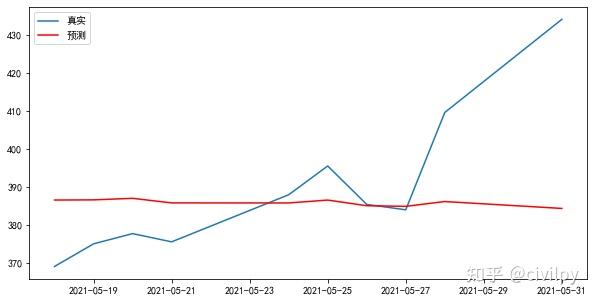
# 预测10天后的股票价格
result = best_arima.forecast(10)
result  # 3个数组分别表示预测值 、 95%置信度的偏差、置信区间
(array([384.36189055, 386.17426305, 384.90800925, 385.07422427,
        386.561561  , 385.80205797, 385.81582908, 387.01726794,
        386.61618881, 386.56756425]),
 array([12.73361992, 19.92899207, 25.41943537, 29.13619276, 33.27661759,
        37.25556235, 40.40642813, 43.81383802, 47.2579767 , 50.20956255]),
 array([[359.4044541 , 409.31932699],
        [347.11415635, 425.23436975],
        [335.08683142, 434.72918709],
        [327.96833582, 442.18011273],
        [321.340589  , 451.782533  ],
        [312.78249754, 458.8216184 ],
        [306.6206852 , 465.01097296],
        [301.14372339, 472.89081248],
        [293.99225649, 479.24012112],
        [288.15862996, 484.97649853]]))
# 构造DataFrame
df_plot= pd.DataFrame(df['close'][:10])
df_plot['predictions']=result[0]
# 绘图
fig = plt.figure(figsize=(10,5))
plt.plot(df_plot['close'],label='真实')
plt.plot(df_plot['predictions'], color='r',label='预测')
plt.legend()
plt.show()

import ffn
result=ffn.calc_total_return(df_plot['predictions'])
ann_result=ffn.annualize(result,10,one_year=250)  # 根据10天数据计算交易日250天的年化收益率
ann_result
0.15379127222659505