数据挖掘之贝叶斯分类
发布时间:2021-12-03
公开文章
# 加载yellowbrick数据集
import os
import pandas as pd
FIXTURES  = os.path.join(os.getcwd(), "data")
df = pd.read_csv(os.path.join(FIXTURES, "spam", "spam.csv"))
df.head()| word_freq_make | word_freq_address | word_freq_all | word_freq_3d | word_freq_our | word_freq_over | word_freq_remove | word_freq_internet | word_freq_order | word_freq_mail | ... | char_freq_; | char_freq_( | char_freq_[ | char_freq_! | char_freq_$ | char_freq_# | capital_run_length_average | capital_run_length_longest | capital_run_length_total | is_spam |
|---|
5 rows × 58 columns
X, y = df.iloc[:,:-1],df.iloc[:,-1]  # 数据集、目标集
df["is_spam"].unique() # 1,0 数字分类,其余因素均为数字
# classes=['not_spam','is_spam']  # 对应 [0,1]
array([1, 0], dtype=int64)
# 分类报告
# visualizer = ClassificationReport(model, classes=['not_spam','is_spam'], support=True)
# 混淆矩阵
# ConfusionMatrix(model,classes=['not_spam','is_spam'],label_encoder={0:"not_spam", 1:"is_spam"})
特征分析
from yellowbrick.features import Rank2D
visualizer = Rank2D(algorithm='pearson')  # 皮尔森相关系数
visualizer.fit(X, y)           # Fit the data to the visualizer
visualizer.transform(X)        # Transform the data
visualizer.poof()              # Draw/show/poof the data
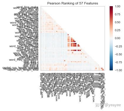
注意强相关的特征并不多
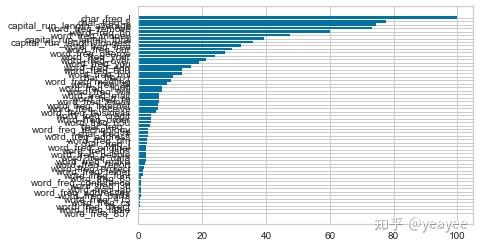
from sklearn.ensemble import RandomForestClassifier  # 分类问题
from yellowbrick.features.importances import FeatureImportances
model = RandomForestClassifier(n_estimators=10)
viz = FeatureImportances(model)
viz.fit(X, y)
viz.poof()
FeatureImportances(absolute=False,
          ax=<matplotlib.axes._subplots.AxesSubplot object at 0x0000025909186F98>,
          labels=None, model=None, relative=True, stack=False, xlabel=None)
rfc = model.fit(X, y)
importances = rfc.feature_importances_
importances
array([0.00419625, 0.00329869, 0.00606181, 0.00068846, 0.02014877,
       0.00599604, 0.05792883, 0.02877044, 0.00333147, 0.00927314,
       0.00606247, 0.01202045, 0.00335088, 0.00115922, 0.00035176,
       0.07424499, 0.02461916, 0.00705513, 0.02264122, 0.00251324,
       0.05250165, 0.00250961, 0.00732771, 0.01208356, 0.06672894,
       0.0112409 , 0.03217723, 0.00360037, 0.00101266, 0.00487104,
       0.00037709, 0.00075526, 0.00115574, 0.00138721, 0.0027788 ,
       0.00204865, 0.01613457, 0.00067385, 0.00496664, 0.00179599,
       0.00153094, 0.00703848, 0.00252604, 0.00217318, 0.00794447,
       0.02254089, 0.0003397 , 0.0008103 , 0.0039666 , 0.01288543,
       0.00291571, 0.08633219, 0.15673341, 0.00346989, 0.05752226,
       0.07943742, 0.03199316])
df1 = pd.DataFrame({'feature':df.columns[:-1],'importances':importances})
df2 = df1.sort_values('importances', ascending=False)
new_features = df[df2[df2['importances']>0.01]['feature'].tolist()]
new_features.shape # 由57个特征降到20个特征,看看结果上的差异  # 事实上用Bokeh也可以实现上面的柱状图
(4600, 20)
分析报告
%%time
from sklearn.model_selection import train_test_split as tts
from sklearn.ensemble import RandomForestClassifier
from yellowbrick.classifier import ClassificationReport

X_train, X_test, y_train, y_test = tts(X, y, test_size =0.2, random_state=10)

model = RandomForestClassifier(n_estimators=10)

visualizer = ClassificationReport(model, classes=['not_spam','is_spam'], support=True)
visualizer.fit(X_train.values, y_train)        # Fit the visualizer and the model
print('得分:',visualizer.score(X_test.values, y_test))        # Evaluate the model on the test data
visualizer.poof()                       # Draw/show/poof the data
得分: 0.9576086956521739
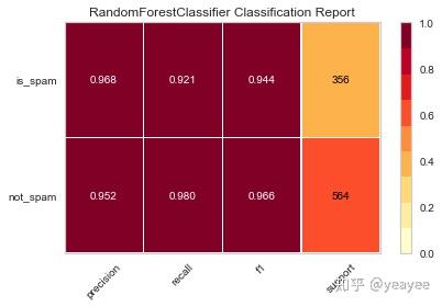
Wall time: 188 ms
%%time
# 新特征20
X_train, X_test, y_train, y_test = tts(new_features, y, test_size =0.2, random_state=10)

model = RandomForestClassifier(n_estimators=10)

visualizer = ClassificationReport(model, classes=['not_spam','is_spam'], support=True)
visualizer.fit(X_train.values, y_train)        # Fit the visualizer and the model
print('得分:',visualizer.score(X_test.values, y_test))        # Evaluate the model on the test data
visualizer.poof()
得分: 0.9391304347826087

Wall time: 176 ms特征降维之后的得分和之前的差异不大
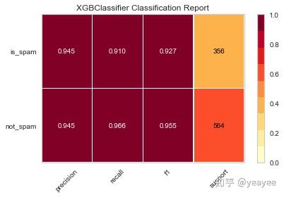
from xgboost import XGBClassifier
X_train, X_test, y_train, y_test = tts(X, y, test_size =0.2, random_state=10)
model = XGBClassifier()
visualizer = ClassificationReport(model, classes=['not_spam','is_spam'], support=True)
visualizer.fit(X_train.values, y_train)        # Fit the visualizer and the model
print('得分:',visualizer.score(X_test.values, y_test))        # Evaluate the model on the test data
visualizer.poof()                       # Draw/show/poof the data
得分: 0.9478260869565217

from xgboost import XGBClassifier
X_train, X_test, y_train, y_test = tts(new_features, y, test_size =0.2, random_state=10)
model = XGBClassifier()
visualizer = ClassificationReport(model, classes=['not_spam','is_spam'], support=True)
visualizer.fit(X_train.values, y_train)        # Fit the visualizer and the model
print('得分:',visualizer.score(X_test.values, y_test))        # Evaluate the model on the test data
visualizer.poof()
得分: 0.9445652173913044
from yellowbrick.classifier import ConfusionMatrix

model = RandomForestClassifier(n_estimators=10)

cm = ConfusionMatrix(model,classes=['not_spam','is_spam'],label_encoder={0:"not_spam", 1:"is_spam"})
cm.fit(X_train.values, y_train)
cm.score(X_test.values, y_test)
cm.poof()
E:\Anaconda3\lib\site-packages\sklearn\metrics\classification.py:182: FutureWarning: elementwise comparison failed; returning scalar instead, but in the future will perform elementwise comparison
  score = y_true == y_pred
整体上差异不大
xgboost 有很多可调参数,具有极大的自定义灵活性。比如说:
(1)objective [ default=reg:linear ] 定义学习任务及相应的学习目标,可选的目标函数如下:
“reg:linear” –线性回归。
“reg:logistic” –逻辑回归。
“binary:logistic” –二分类的逻辑回归问题,输出为概率。
“multi:softmax” –处理多分类问题,同时需要设置参数num_class(类别个数)
(2)’eval_metric’ The choices are listed below,评估指标:
“rmse”: root mean square error
“logloss”: negative log-likelihood
(3)max_depth [default=6] 数的最大深度。缺省值为6 ,取值范围为:[1,∞]